Blog

There are several ways to identify duplicate data in Excel. We can either use helper functions, or Excel’s own inbuilt options such as conditional formatting or pivot tables.

We will look at each of the following

• Functions to identify duplicates
• Formatting to identify duplicates
• Pivot tables to identify duplicates

Consider the following dataset, we wish to identify any Ticket IDs which are duplicates.

Using Functions to identify duplicate values

We can use functions in helper columns to help us identify duplicate data. The functions we can use are based on arrays which we should first understand.

You can skip directly to using the functions, or understand how these functions work as follows.

• SUMPRODUCT to identify duplicates
• COUNTIF to identify duplicates

Background to Arrays

In computing, an array is a ‘set’ of data values.

We also refer to a scalar value, which is a single unit of data, such as a number. So an array is typically a collection of scalar values.

In Excel this could be a set of values, or a reference to values, such as a column range, or row range, or multiple rows or columns.

Excel uses the “{…}” notation in functions to indicate an array.

NOTE: A cell range is a reference to an array of cell values.

A simple array example

If we have 5 scalar values: 1, 1, 2, 2, 3 – we can form these into an array (or ordered collection) as follows

{1,1,2,2,3} 

We want to compare each value in the array to a specific scalar (e.g. ‘2’) and sum all the matching values to give us a total.

{1,1,2,2,3} = 2 

Each value of the array, is equated independently to the scalar. The result is another array of Boolean (TRUE or FALSE) values,

The value will be TRUE where the array item was equal to our scalar value, otherwise FALSE, in the corresponding position in the array.

={FALSE, FALSE, TRUE, TRUE, FALSE}

NOTE: An interesting property of Booleans in Excel is that TRUE is equivalent to the value 1 and FALSE to the value 0.

However we cannot easily sum TRUE values, as this would give an error, but we can sum their numerical equivalent value (ie 1 or 0). To do this we have to force excel to use their numeric equivalent.

This can simply be done by multiplying the array by 1

{FALSE, FALSE, TRUE, TRUE, FALSE} * 1

which outputs and array of numerical values which can then be summed

{0, 0, 1, 1, 0}

The array of numeric values can now be summed to give you the sum of TRUE responses. You can check this out in Excel as a function.

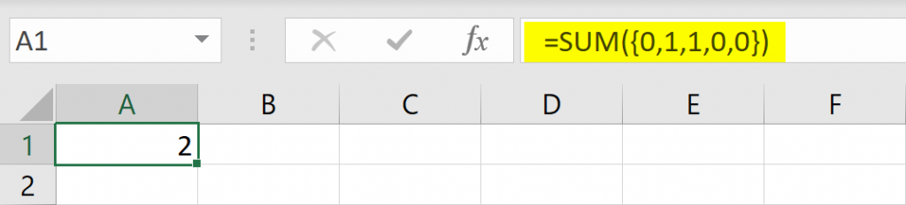
=SUM({0,0,1,1,0})

which gives

2

Putting it all together with our array example data, we get the same answer as before when identifying the number of 2s in our number array.

Identifying Duplicates with Excel functions

So how does that help us find duplicates? Well we can test each of our data values against all the other values (who’s cell range will form an array) and we can count the number of items equal to the comparison value. We will do this for each value in our dataset. Where the value is unique we will get 1 returned otherwise we will get the number of matching occurrences (or duplicates).

So with our test data, if we create a helper column and test each row against the ‘Ticket ID‘ range, we will get the number of duplicates for any inputted value.

Using SUMPRODUCT

Typically the SUMPRODUCT function is used to sum the products of similarly sized (or dimensioned) cell ranges.

In its most basic definition the SUMPRODUCT function is defined as follows, where each array is of the same dimension.

=SUMPRODUCT(array1, [array2], [array3], ...)

Each array (or range of cell values) is multiplied against the other array values before being summed, and a single scalar value output (being the sum of the product of the arrays).

Extending SUMPRODUCT

We can use the array functionality of SUMPRODUCT to compare any particular value with a range of input values.

The array property can be used to identify duplicates by comparing any specific value in the dataset against all values in the dataset.

How it works

1. Select the range of data values in Column A (that is A2:A13)
2. Use the shortcut F4 or ‘$‘ symbol, to convert the range to a fixed range in the formula, i.e. $A$2:$A$13
3. Equate the range to the value in the same row (without fixing this value), in row 2 we select Cell A2
4. put parenthesis around the array evaluation, before multiplying by 1, so that the array is evaluated first.
5. Press Enter to evaluate the function in B2.
6. Drag or copy the function from B2 to B13, to compare against all Ticket ID values, the initial value A2 will update to correspond to the row of the function while the dataset cell range remains fixed.

Here we see that

• AB1002, AB1006, AB10007 and AB1011 are unique with only 1 instance each, so are non duplicated values.
• AB1001 and AB1005 have 3 instances (occurrences),
• AB1009 has 2 instances in our data.

We can filter the SUMPRODUCT value to find those values with duplicates.

NOTE: Since Excel 2010, New array based functions have been added to Excel, in particular COUNTIF.

COUNTIF for this particular example is more straight forward, However for versions of Excel prior to the introduction of COUNTIF, eg Excel 2003, the SUMPRODUCT option above is how you can identify duplicates.

Using COUNTIF

With COUNTIF we supply a cell range, and a value, without having to convert Boolean arrays to numeric values.

COUNTIF is another array based formula, where range is a range of cells.

=COUNTIF(range, criteria)

How it works

By selecting the function and clicking the INSERT FUNCTION shortcut “SHIFT + F3” we can see how our function works. The range argument is actually converted to an array by the COUNTIF function (note the “{…}” brackets), highlighted, before being evaluated against the selection criteria.

The only difference between the SUMPRODUCT method and COUNTIF, is that the Boolean array does not have to be explicitly converted to numeric values before being aggregated in the COUNTIF function.

Using Conditional Formatting to identify duplicate values

With more recent versions of Excel we can also identify duplicated values with Conditional formatting. In this case we don’t need a helper column at all, or the need for functions.

• Select the dataset
• On the HOME Ribbon, select Conditional Formatting button/drop-down
  • Select Highlight Cells Rules
  • Select Duplicate Values
• From the pop-out Duplicate Values window, accept the Duplicate value in the dropdown.

The original dataset will now be color formatted showing duplicated values in Red (or other option as selected).

Using Excels Filter option allows you to filter on cell color, should you wish

Bonus – Conditional Formatting – Unique Values

You might have noticed the dropdown option in the Duplicate Values formatting window. If you select Unique from the dropdown instead of Duplicate, you will get only those values with non-duplicate entries formatted. This could be a great way of only selecting non duplicated data.

Here I also selected the alternative Green Fill with Dark Green Text option.

Excel’s Sort & Filter option allows for filtering cells by formatting as well as by value. Only current formatting will be options to select from, either by font color or by cell color.

In our example, filtering by Cell Color, will allow only the truly unique values to be filtered filtering out duplicated values.

Using Pivot Tables to identify duplicate values

Pivot tables are great in as much as they are both powerful, but can be controlled largely with drag and drop functionality.

Pivot tables also easily aggregate similar values on grouped data, to allow numerical analysis such as SUM and COUNT.

We can use this simple fact to identify both unique values (by grouping values) and count data in each group.

Duplicate values will return a ‘count’ value greater than 1.

1. Select the data in the list, or table
   1. in our case our list is the range A1:A13 (including the header)
2. Click on the Pivot Table button in the Ribbon’s INSERT menu
3. Accept the default option to create a new pivot table in a new worksheet
4. A blank pivot table is created, on the right you can see the fields (column headers) available from the initial selection,
   1. click and drag the “Ticket ID” field into the Rows box in the bottom left.
   2. repeat the click and drag of the “Ticket ID” from the same initial field list, this time dropping it into the bottom left Values box

How it works

The result of dragging the Ticket ID field into the Rows box will populate column A of the pivot table with all values in Ticket ID, grouping each.

The result of dragging the the Ticket ID field into the Values field will initially default the values to being counted in the data field (or column B of the Pivot Table) for each unique value in the Rows field.

The result is that we can see again that:

• AB1002, AB1006, AB1007 and AP1011 all have only one occurrence each,
• while AB1001 and AB1005 have 3 occurrences in our original data and
• AB1009 has 2 occurrences.

In conclusion we have a variety of ways to inspect our data in Excel (without reference to VBA – which offers further options). Which you choose will depend on how you are analysing or visualising your data.

Dealing with multiple column duplicates

Finally, when dealing with multiple column duplicates, one way we can analyse this with the methods above is to first create another helper column and concatenate all the values into a single new value.

Then we can simply repeat any of the processes previously listed above on the new concatenated field.

NOTE: It is a good idea to split the concatenated values with a delimiter, in this case “:” was chosen, since there are times when 2 independent values combined can equate to the same value otherwise. Eg “1 & AB” and “1A & B”.

Using a delimiter which otherwise would not appear in your values, such as “:”, “::” or “|” will reduce any such potential issue.

048